Web Queries allow you to automatically push Marin data into your Google sheet. Anytime you open the Google Sheet, you will have access to the latest data.
For Excel users, see Web Query Reports in Excel
Setting Up Web Query Reports For Google Sheets
- The first step is to create your web query following the instructions in our dedicated article. Specifically, check out the Creating Your Web Query Report in Marin section.
- Once you've generated your web query report, in the Left Navigation Bar, under Reports select Scheduled.
- From here, use the File column and click on the blue icon to copy your web query URL.
- Open your Google Sheet in a new browser tab.
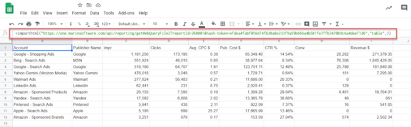
- Click into a cell and type
=IMPORTHTML(
This function / formula imports data into a Google Sheet from a table within a HTML page. - Next, you'll add the syntax.
=IMPORTHTML("url", "query", index)-
url refers to the URL of the page to be examined and should include the protocol (e.g. https://).
This is where you will paste the web query report URL that you generated in Marin. Be certain your URL is enclosed in quotation marks. -
query can be either "table" or "list", depending on what type of structure contains the data.
For Marin’s web query reports, we'll use the query "table". Be certain this is enclosed in quotation marks -
index refers to a number, beginning at 1, and identifies which table or list should be returned, as defined in the HTML source code.
For Marin's web query reports, there are three tables to choose from, as shown in the image below. This number does not need to be enclosed in quotation marks, unlike the URL and query.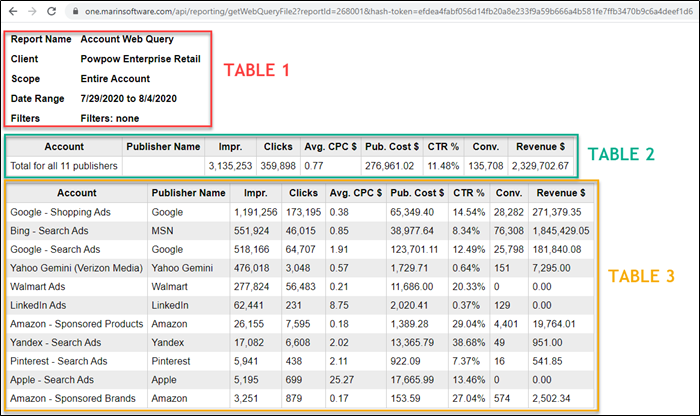
-
url refers to the URL of the page to be examined and should include the protocol (e.g. https://).
- Your finished formula should look similar to the example below, with a URL that is specific to your web query. Make sure that each piece of syntax is separated by a comma.
=IMPORTHTML("https://one.marinsoftware.com","table",3)
- After you enter your entire formula, including syntax, hit Enter on your keyboard. Once you hit enter, the data will be imported into the Google Sheet from your web query report.
- When your data has been populated, you'll have the opportunity to set the criteria that will be used for the report to refresh.
To do this, from your Google Sheet, click File and select Spreadsheet settings. In the pop-up, click Calculation and change the recalculation to On change and every hour. Then, click Save Settings.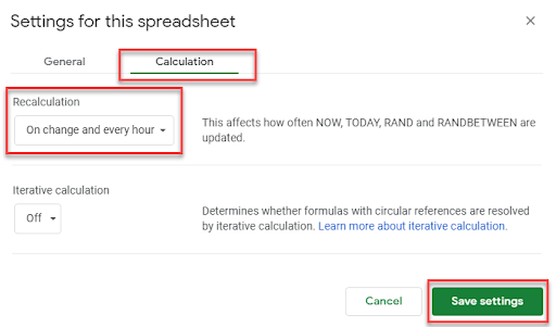
- Google will now automatically refresh the data on an hourly cadence, so you can be sure that the most recent data is up-to-date -- there’s no need to manually refresh, like in Excel.
That's all there is to it!
Google Sheets vs Excel
There are a few benefits to using Google Sheets instead of Excel, including a built-in revision history, auto-save functionality, and a real-time chat window so you can communicate with your colleagues about your report data. And, due to the Cloud-based nature of Google Sheets, collaboration between multiple users makes a marketers workflow easier and faster. Additionally:
- You can access your Google Sheet and corresponding data from any computer, without needing to download additional software.
- Refreshing your data takes place automatically, on an hourly cadence -- no manual intervention needed.
- You have control over data access levels, including Read-Only, Edit, or Comment access.
- You can share data easily with management and stakeholders.
- The data can also be synced into Big Data Tools from Google Sheets for enhanced customization and reporting using Google Data Studio.
- The pricing can't be beat – Google sheets is completely free to use.
We'll walk through how to import your web query into Google Sheets below.
